Valuing Uniswap V3 Liquidity Positions#
This guide walks through the process of querying a Uniswap V3 pool from an on-chain state
Setting up Simulation#
import logging

import numpy as np
from tqdm import tqdm
from matplotlib import pyplot as plt
from web3 import Web3
from eth_utils import to_checksum_address

from nethermind.entro.base import PoolFactory
from nethermind.entro.uniswap_v3 import UniswapV3Pool

LIQUIDITY_SNAPSHOT_BLOCK = 14000000
LP_POSITION_MANAGER = to_checksum_address("0xC36442b4a4522E871399CD717aBDD847Ab11FE88")

pool_factory = PoolFactory(
    sqlalchemy_uri=f"postgresql://user:pass@host/db_name"
    w3=Web3(Web3.HTTPProvider("https://localhost:8545", request_kwargs={"timeout": 60})),
    logger = logging.get_logger("position_simulations")
)
Querying Historical Pool States#
Caching Pool States
Through the load_pool() and save_pool() methods, the on-chain query results can be cached. This reduces the setup time for a pool from 10-40 minutes to a few seconds.
def initialize_pool(pool_factory, pool_address, at_block) -> UniswapV3Pool:
    if os.path.isfile(f"pool_states/{pool_address}_{at_block}_pool_state.json"):
        with open(f"pool_states/{pool_address}_{at_block}_pool_state.json", "r") as f:
            return UniswapV3Pool.load_pool(f, pool_factory)

    else:
        pool = pool_factory.initialize_from_chain(
            pool_type="uniswap_v3",
            pool_address=to_checksum_address(pool_address),
            at_block=at_block,
        )
        with open(f"pool_states/{pool_address}_{at_block}_pool_state.json", "w") as f:
            pool.save_pool(f)

        return pool
>>> usdc_weth_pool = initialize_pool(pool_factory, "0x88e6A0c2dDD26FEEb64F039a2c41296FcB3f5640", LIQUIDITY_SNAPSHOT_BLOCK)

# Verify that pool is initialized correctly
>>> usdc_weth_pool.immutables.fee
500
Simulating Pool Activity#
Now that we have a pool state initialized, we can simulate ppool swaps and analyze their impact on individual positions, and the greater pool state.
Simulating Synthetic Swap Dataset#
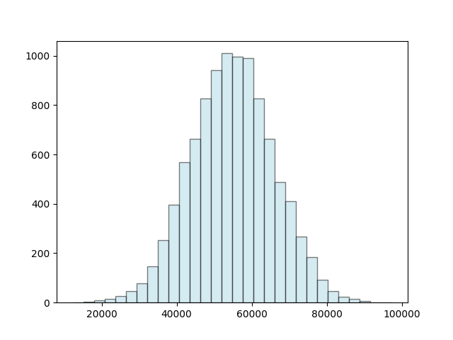
>>> TRADE_COUNT = 10_000  # Number of Swaps to Simulate
>>> MAX_TRADE_SIZING = 100_000  # Max Trade Size in USD
>>> MIN_TRADE_SIZING = 10_000  # Min Trade Size in USD

>>> normal_distribution = np.random.normal(0, 0.2, TRADE_COUNT)
>>> trade_range = (MAX_TRADE_SIZING + MIN_TRADE_SIZING) / 2

>>> trade_amounts = []
>>> for datapoint in normal_distribution:
...    trade_amounts.append(trade_range + (datapoint * trade_range))

# Plot the trade sizing
>>> plt.hist(trade_amounts, bins=30, alpha=0.5, color="lightblue", edgecolor="black")
>>> plt.show()

The next step is to convert these USD trade sizes into raw token_0 and token_1 amounts, and execute the swaps on the pool
>>> for index, trade_amount in enumerate(tqdm(trade_amounts)):
...    swap_direction = np.random.choice([0, 1])
...    sqrt_price_limit = TickMathModule.MIN_SQRT_RATIO + 1 if swap_direction else TickMathModule.MAX_SQRT_RATIO - 1
...    amount_specified = int(trade_amount * (10 ** 6) * (1 if swap_direction else -1))
...    pool.swap(amount_specified=trade_data, swap_direction, sqrt_price_limit)
...    pool.advance_block(4)
...
...    # Every 50 swaps, log position valuations to the database
...    if index % 50 == 0:
...        pool.save_position_snapshot()
Getting Historical Pool Swaps#
Note
This Process is in the process of being automated with improved UX. This is currently possible by scraping swap events starting at the pool_initialization block, and going forward a few months.
Visualizing Position Valuations#
Note
USD Position Valuation is in the process of being implemented.
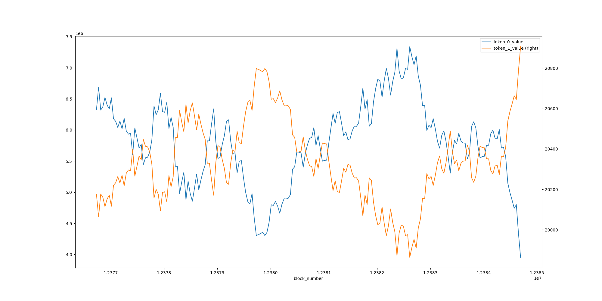
>>> active_position = usdc_weth_pool.get_position_valuation(LP_POSITION_MANAGER, 194890, 195510)

>>> active_position

     block_number  token_0_value  ...  token_1_value_usd position_value_usd
0        12384693   3.953397e+06  ...               None               None
1        12384653   4.339269e+06  ...               None               None
2        12384613   4.800521e+06  ...               None               None
3        12384573   4.742173e+06  ...               None               None
4        12384533   4.874176e+06  ...               None               None
..            ...            ...  ...                ...                ...
195      12376893   6.523035e+06  ...               None               None
196      12376853   6.374573e+06  ...               None               None
197      12376813   6.320359e+06  ...               None               None
198      12376773   6.687767e+06  ...               None               None
199      12376733   6.326365e+06  ...               None               None
[200 rows x 6 columns]


>>> fig, ax = plt.subplots(figsize=(20,10))
>>> pos_1.plot.line(x="block_number", y="token_0_value", ax=ax)
>>> pos_1.plot.line(x="block_number", y="token_1_value", secondary_y=True, ax=ax)
>>> plt.show()
